Spis treści

How this work was done

Below are the overall steps taken:

Signal collection
Burst extraction
Timing offset estimation
Frequency adjustment
Phase adjustment
OFDM symbol extraction
Scrambler generation and application

Information Known Ahead of Time

There were some very important parameters that were known going in:

Occupied bandwidth: ~ 10 MHz
Modulation type: OFDM
Burst duration: Very short (no actual number initially, just that it was only a few OFDM symbols)
Frequency: Somewhere in 2.4 GHz

It was also known that the signal looked a lot like LTE, and used some LTE features. What that ended up meaning is that the actual signal bandwidth was 15.36 MHz (LTE downlink signals with an occupied bandwidth of 10 MHz are actually 15.36 MHz wide [1].)

Also, the signal was known to come from the drone and not the controller

[1] https://www.sharetechnote.com/html/Handbook_LTE_PhyParameter_DL_FDD.html

Signal Collection

I used a DJI Mini 2 for my analysis. Please keep in mind that not all drone models or firmware versions are always going to generate the same signal structure!

Once the drone was registered and powered on, I used GNU Radio with gr-fosphor to hunt for the Drone ID signal. To help with reducing unwanted interference I placed the SDR next to the drone with the RX gain set low, and the controller in another room. Then I scrolled through 2.4 and 5.8 GHz looking for signals that were 10 MHz wide and bursty.

What I found from that was that there were a handful of frequencies that matched the description:

2.4595 GHz
2.4445 GHz
2.4295 GHz
2.4149 GHz
2.3995 GHz

This is likely not an exhaustive list, and I've heard that some drones also send DroneID in 5.8 GHz.

One issue with recording Drone ID is that it transmits very infrequently (about every 640 milliseconds), and hops around from frequency to frequency (see the list above). So, if you want to capture bursts you might have to record for several minutes, which at a sampling rate of 15.36 MSPS (more on this later) is 61.44 MBytes per second for complex shorts, or 128.88 MBytes per second for floats. A better way to do this is to record only when the signal is active on the current frequency. This can be done easily with osmocom_fft from gr-osmosdr [2] using gr-fosphor [3]. The use of gr-fosphor is important here as the normal FFT that you get by running osmocom_fft isn't going to update fast enough to see very short (in time) bursting signals. Using gr-fosphor will allow you to see those bursts that the normal FFT will miss. But, this does require either a GPU or and OpenCL supporting CPU.

Unfortunately for me, gr-fosphor was not playing nice with my computer when running under Qt, so that made osmocom_fft -F useless for my case. So, I wrote a GNU Radio flow graph (see below) that allowed me to choose when to start recording by pressing and holding a button in the Qt UI.

Some things of note about the graph:

The sample rate is twice the required rate to make the recording as accurate as possible. When trying to reverse engineer a signal, it's best to record at the highest sampling rate you reasonably can so long as you don't have to sacrifice dynamic range (ie. drop to a lower sample size)

The output file is going to /dev/shm. You need to be able to write the samples to a file as fast as they are coming in. As mentioned earlier, the data rates involved in recording high sample rate signals can be a bit too much for a normal hard drive. So, to ensure that disk IO does not cause samples to be dropped, /dev/shm is used as it maps directly to RAM without having to touch the hard drive. If you have a sufficiently fast NVMe drive, and the OS isn't using it actively, then you can try that too. Do be aware that if you fill /dev/shm up, your OS might start doing strange things as some applications (Google Chrome for example) use /dev/shm to store temporary files.

So, using that graph I was able to collect several frames with the files stored in /dev/shm.

[2] https://github.com/osmocom/gr-osmosdr

[3] https://github.com/osmocom/gr-fosphor

= Burst Extraction With a recording in hand, it's time to find when the burst starts and how long it's active for. To view signals this way I prefer to use baudline [4]. It's an amazing tool considering it's free.

Heads up: The images below are going to have tiny font settings. This is an issue with baudline on HiDPI displays and I don't have an easy fix. So apologies in advance!

Before opening the collected file, run baudline, right click in the main window, and select Process -> Transform Size and click 65536. This needs to be done if your file is over a few hundred MBytes or the app will just crash after trying to open the file.

Now right click in the main window again and select Input and click Open File. The navigation menu is very old school. The left side is directories, and the right side is files. Navigate to where you saved the collect using the left pane, and the select the file by clicking it once in the right pane. Then make sure that the File Format dropdown is Raw and click Open. Failing to change the file format will result in an error when you click Open

A new window will pop up with the signal parameters. From top to bottom:

Decompression: Auto Magic
Initial Byte Offset: 0
Sample Rate: Change to Custom and enter the sample rate (in Hz) of your collected file (mine was 30720000)
Channels: 2 and check both Quadrature and Flip Complex
Decode Format: This will depend on how you collected the signal. If you used osmocom_fft or my graph example then this will be 32-bit float. If you used the HackRF command line tool, then this might be 8-bit linear (signed). Otherwise it's going to be 16-bit linear as that's really the only other common sample size. Do not change the endianness unless you really know what you're doing!
Normalization: auto measure

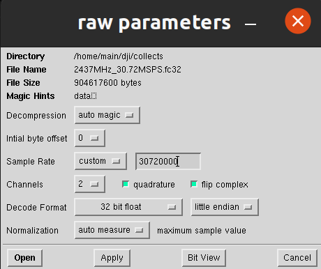
Click on Open and the popup should go away and the main window should update with something similar to the following

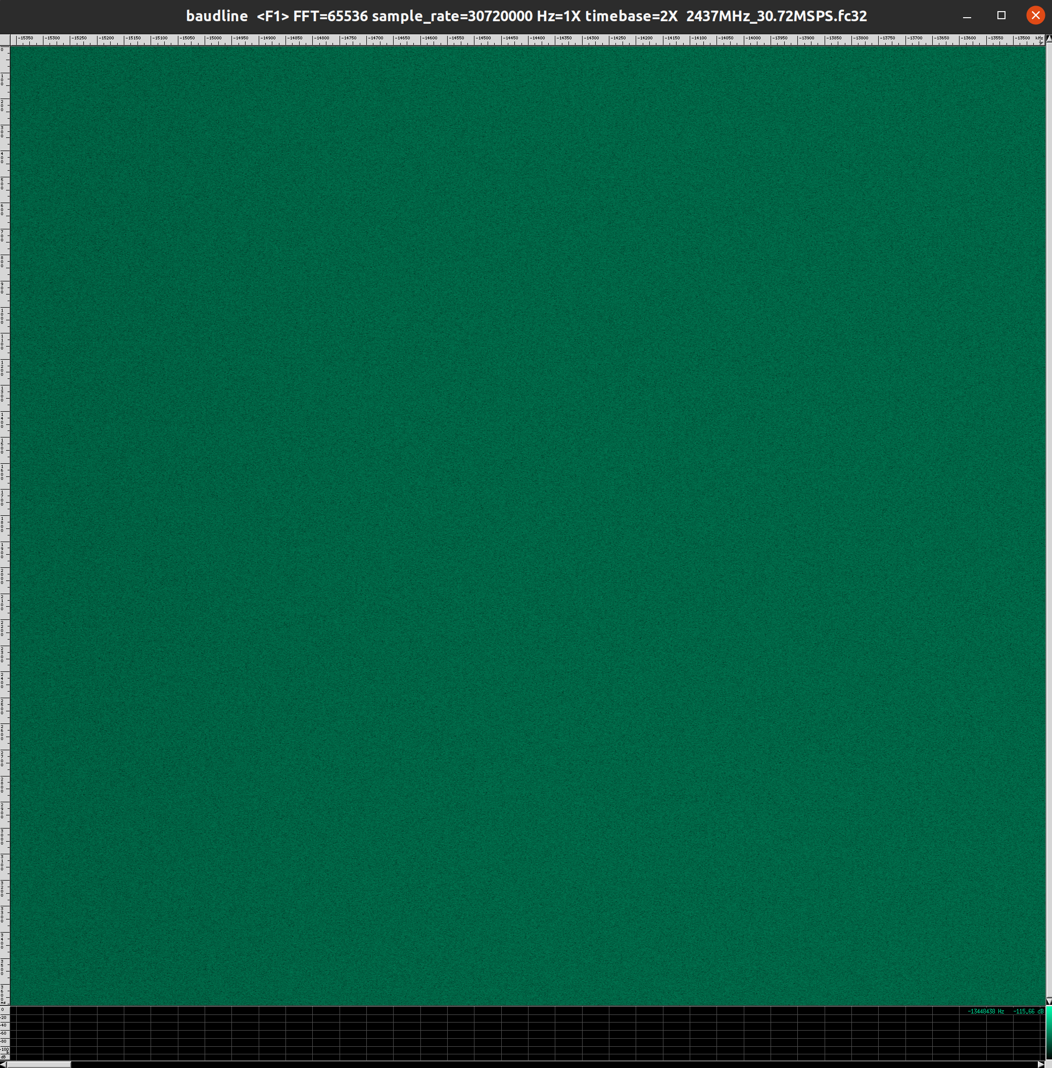
The first thing to do is fix the FFT size. Right click in the main window, select Processing -> Transform Size, and select 4096. Dropping the FFT size is fine now that the file is loaded. Any size over 4096 usually results in having to scroll left and right to see the full bandwidth.

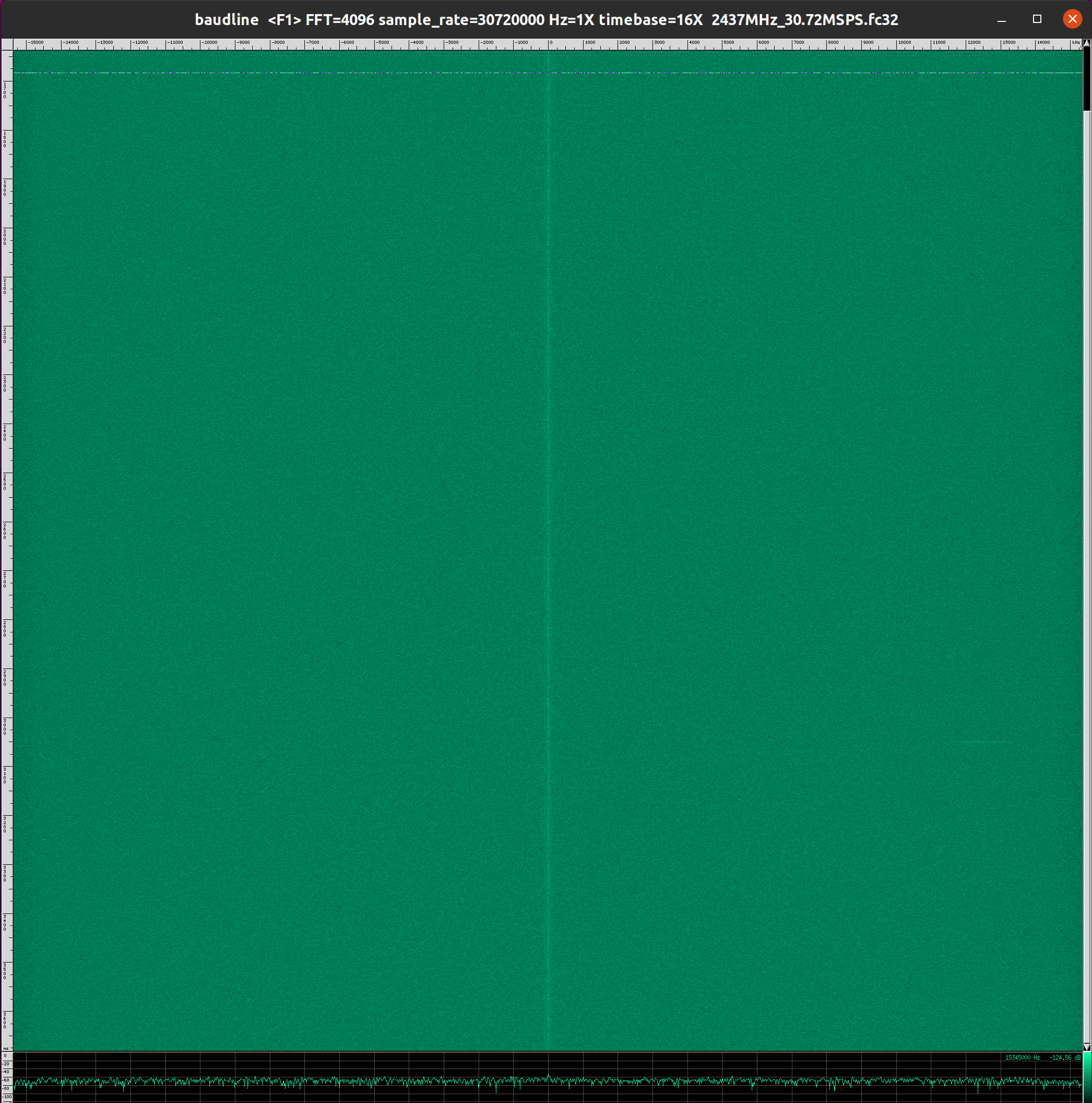
In my case the collect was long enough that baudline didn't show my anything useful at first. This happend because baudline zooms you all they way out at first. So you're seeing the entire collect in one window. To zoom in press alt and scroll forward with the mouse wheel (might be the windows key for some window managers). You should hopefully see something like this after scrolling and zooming around

That is a DroneID burst!

The important information that we need now is when does the burst start, and how long does it stay active. Handily, baudline gives us tools for doing just that. Right click in the main window and select measure -> system and select delta selected, then go to the same menu again and select cursor time.

By default the windows might be absolutely tiny. If they are, click on one of them and press the up arrow until they are the correct size

You should now notice that moving the mouse vertically in the main window changes the time value in cursor time. If you click and drag vertically you will notice the values in delta selected changing.

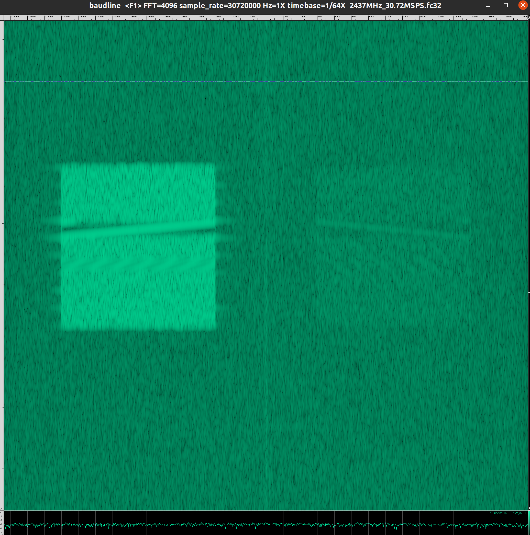
Find a burst that looks like the image from earlier, and click just above it in the main window. Clicking will lock the cursor in place. Note the time that the burst starts.

Now, click and drag until you have highlighted the entire signal (going over is fine) and note the value of delta selected

You now know when the burst starts in the collect, and for how long it stays active. This will be used in later steps to extract just the samples that you care about.

Burst Extraction

Now that you have an idea of when the bursts starts in time and how long it stays up, the samples that make up that time period can be extracted and analyzed further.

What follows will be MATLAB code, but should work fine in Octave as well.

First you need a way to read the samples into MATLAB. To the best of my knowledge there is no simple read_complex_samples function in MATLAB. But, there is an Octave function provided by GNU Radio that works fine in MATLAB [4]. I have my own version [5] that I used for this work.

So, regardless of which method you want to use to read in samples, you first need to figure out what the sample offset is given the time offset you figured out from earlier.

Continuing from the example above, the file was recorded at 30.72 MSPS (2x oversampled), so just multiply the sampling rate by the time offset to determine the sample offset. Do the same to determine how many samples the signal is active for. This means:

sample_rate = 30.72e6;

start_time = 2.722209;
burst_duration = 0.00080729;

start_time_samples = round(start_time * sample_rate);
burst_duration_samples = round(burst_duration * sample_rate);

fprintf(1, 'Start sample offset: %d, sample duration: %d\n', start_time_samples, burst_duration_samples);

Running this script you should get the following output:

Start sample offset: 83626260, sample duration: 24800

Next the samples need to be read from the file they were recorded to. Using the function in [5] that looks like this:

file_path = '/path/to/your/file.fc32';
sample_rate = 30.72e6;

start_time = 2.722209;
burst_duration = 0.00080729;

start_time_samples = round(start_time * sample_rate);
burst_duration_samples = round(burst_duration * sample_rate);

samples = read_complex_floats(file_path, start_time_samples, burst_duration_samples);

length(samples)

The output of which should look like:

ans =  24800

Which means that samples now contains 24,800 complex samples.

Now that you have the samples, it's a good idea to plot them to make sure that you really got a full burst. An easy way to do this is to plot the magnitude squared (abs(samples).^2). Add the following to the script above:

figure(1);
plot(10 * log10(abs(samples).^2));

In my case the plot looks like this

Plotting in log scale to make the small variations stick out, and to get a sense of the signal to noise ratio of the recording.

You should see nothing, and then a signal appearing, and then dissapearing before the end of the samples. If you have caught the signal too early, or don't see the end of it, then you need to go back to baudline and double check your measurements. If it's still not working, make sure that when you open the file in baudline that you specify the correct sampling rate. If that value is wrong, then the time information that baudline gives you will be incorrect as well.

At this point you have successfully extracted a single burst. Now it's time to move on to figuring out exactly which sample is the first sample of the burst.

Your MATLAB code should look like this (obviously changing the path, sample start time, and burst duration values)

file_path = '../collects/2437MHz_30.72MSPS.fc32';
sample_rate = 30.72e6;

start_time = 2.722209;
burst_duration = 0.00080729;

start_time_samples = round(start_time * sample_rate);
burst_duration_samples = round(burst_duration * sample_rate);

samples = read_complex_floats(file_path, start_time_samples, burst_duration_samples);

figure(1);
plot(10 * log10(abs(samples).^2));

[4] https://github.com/gnuradio/gnuradio/blob/main/gr-utils/octave/read_complex_binary.m

[5] https://github.com/proto17/dji_droneid/blob/main/matlab/read_complex_floats.m

Timing Offset Estimation

This is where the DSP is going to get a bit heavier :)

We know ahead of time that this is an OFDM system. That means that there are going to be symbols that consist of some number of samples, and a cyclic prefix that comes before each symbol. While it's not important to understand why there is a cyclic prefix, or why OFDM is used. Just the following:

The cyclic prefix is nothing but a copy of the last N samples of the symbol. It's literally copy pasting the last N samples of the OFDM symbol and prepending them to the symbol

As an example, if the OFDM symbol is 512 samples long, and the cyclic prefix is 16, then the resulting full OFDM symbol is 512 + 16 or 528 samples long.

You can actually see this in the plot from earlier. If you look closely about 1/3 of the way into the burst you will see that one chunk of time looks like it's symmetrical:

The image above is zoomed into the symmetrical part. For illustrative purposes I have drawn colored boxes over the areas that are not a part of the OFDM symbol + cyclic prefix

This should look somewhat asymmetrical, like something was added to the beginning (because it was!). Below I have highlighted the cyclic prefix in a different color.

You should now be able to see that the newly highlighted samples look a lot like the last few samples that aren't highlighted. This feature is almost always present in OFDM systems, but isn't always this obvious. And as we will discuss later, not all OFDM symbols are symmetrical like this (special feature of this specific OFDM symbol)

One other piece of knowledge about OFDM symbols: They are very commonly a power of 2 in length

This isn't always the case, but a power of two means that a Fast Fourier Transform (FFT) can be used instead of a Discreet Fourier Transform (DFT) - the latter being more computationally expensive.

Taking a look at the samples in the plot from earlier we can roughly calculate the number of samples in each symbol. This symmetrical symbol will be the easiest to work with since the boundaries of the symbol are more obvious than the others. Looking at the MATLAB plot we can see that the left-most sample in the white box is about 7,700 and the right most is about 9,760. The difference of the two being 2,060 which is very close to 2048 which is a power of 2 (2^11).

These numbers were determined by moving the mouse in the plot and looking at the bottom left at the X axis coordinate for the left and right sides of the white box (the one that wasn't colored).

This means that the FFT size is almost certainly 2,048 samples. The cyclic prefix length is a little harder to guess as it doesn't need to be any specific multiple. Thankfully we know that the signal supposedly follows LTE, so that value is known.

Assuming for a moment that the cyclic prefix length is not known, there are ways to find it. You can take advantage of the fact that the cyclic prefix is a repeat of the last N samples of the OFDM symbol. You can use autocorrelation over a range of samples and values of N to figure out which value of N ends up with the highest correlation score. It's a little out of scope here as we know that the signal follows some of the LTE spec.

Going back to [1] you can see that for a signal that occupies 10 MHz of bandwidth (as this signal does) the FFT size should be 1024. But we have 2048... What gives? Oversampling

The recording was taken at 30.72 MSPS, while the signal only needed to be recorded at 15.36 MSPS. This doubles the number of samples, and for OFDM systems means that our FFT size and cyclic prefix lengths are doubled in the recording we made. This doesn't cause any issues thanks to how an FFT works.

So, since the file was oversampled by 2x we are going to use an FFT size of 2048. As for the cyclic prefix, well, there are two lengths:

Long
Short

The chart in [1] shows that the long cyclic prefix should be 5.2 microseconds, and the short prefix 4.69 microseconds. Multiplying the sample rate with the cyclic prefix duration in seconds will give you the number of samples:

30,720,000 * 0.0000052 = 159.744 or 160
30,720,000 * 0.00000469 = 144.0768 or 144

According to the LTE spec, the first OFDM symbol should use the long cyclic prefix, but the remaining symbols in the slot use the short cyclic prefix.

So, lets check to see if this math works out. From the MATLAB plot earlier the OFDM symbol seemed to end (far right of the white box) around sample number 9,760. Assuming that each symbol after the first is 2048 + 144 or 2192 samples, the end of the previous OFDM symbol should be 9760 - 2192 or 7,568

The mouse cursor is roughly at 7,568 and that does look like the very beginning of the OFDM symbol from earlier. Subtracting 2,192 again gives 5,376

Moving back again by 2,192 gives 3,184

For the next symbol the cyclic prefix length should be 160, so we need to subtract 2048 + 160 or 2208 which gives 3184 - 2208 or 976

NOTE: The screenshots aren't putting the mouse cursor where it actually is. In the screenshots the cursor is several pixels to the left of where it truly is. While it may look like the cursor is before the burst, it isn't actually!

And that brings us back to the very beginning of the burst! We can assume that a rough starting sample for the burst is 976. We will have to refine this value further in order to demodulate, but it's a starting point, and validates the expected cyclic prefix and FFT size assumptions.